Qiskit: Running Quantum Programs

You have already learned how to create Quantum Circuits using Qiskit. In this chapter of the Qiskit Tutorial, you will learn how to run your Quantum Program. You will be running these programs on a Classical Machine which will simulate an Error Correcting Quantum Computer. Though no Error Correcting Quantum Computer exists anywhere in the world today, it is expected that they will soon be a reality. In later chapters of this tutorial you will also run your Quantum Program on an actual Quantum Computer by IBM.

---

Running a Quantum Program

You will now create a Quantum Program and run it on a simulator on your local machine.

Qiskit Aer

Qiskit Aer provides an interface to run Quantum Programs locally on your machine. Therefore Aer needs to be imported first.

# Importing Aer
from qiskit import Aer

Qiskit Aer provides a interface for many backends which simulate a Quantum Computer. These backends can be explored by calling the backends() function on Aer.

Aer.backends()

This will output the list of available backends.

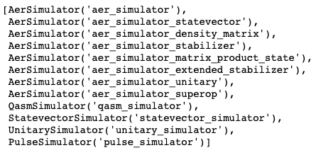
In this chapter, we will be making use of Aer Simulator(class AerSimulator).

Creating Quantum Circuit

Additionally, we also need to import the QuantumCircuit class which is needed for building Quantum Circuits.

# Importing QuantumCircuit
from qiskit import QuantumCircuit

Next, we will create a Quantum Circuit with one Qubit and one bit.

# Creating a Quantum Circuit with 1 Qubit and 1 bit
qc = QuantumCircuit(1, 1)

# Measuring the value of Qubit onto classical bit
qc.measure(0, 0)

Note– The state of the Qubit is by default initialized to 0. In this Quantum Program we are just measuring the state of the Qubit.

Running Simulation

Everything is set for running the Quantum Program we just built. To run the quantum program, first choose a simulator.

simulator = Aer.get_backend('aer_simulator')

Next, we run the program on the Simulator and get the results.

result = simulator.run(qc).result()

result contains information about the program that was just run on the Simulator. The simulator runs the Quantum Program a given number of times, by default 1024. The number of times the Quantum Program needs to run can be passed to the run() function as shots parameter. The number of times the measurement of Qubit results in 0 and 1 is returned by the get_counts() function.

counts = result.get_counts()

The output of get_counts() for this example is-

Note– Notice that the result of running the program 1024 times results in 0 all the times. This is what was expected, because the Qubits are initialized in the |0> state, and no operation was performed on the Qubit before measuring it. Hence, the measurement will result in 0 every time.

You can initialize a Qubit into any state you want. _{Learn more about Initializing a Qubit}

Visualizing the Output

The output of the Quantum Program can be vizualized in various forms such as Histograms, Q-Sphere, CityScape, etc. You will be learning about plotting various vizualizations by using Qiskit in a later chapter. In this chapter, we will just be vizualizing the outputs with the help of a histogram.

To plot histogram, plot_histogram() function needs to be imported from qiskit.visualization

# Importing plot_histogram function
from qiskit.visualization import plot_histogram

Next, pass the the counts variable to plot_histogram() function. This will plot the histogram for the outputs of the Quantum Program.

plot_histogram(counts)

The output of this will be-

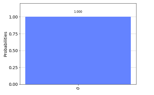
Note– As discussed above, the Qubits are initialized in state |0>. Hence, measuring a Qubit without performing any operation will always result in 0. For this reason, the probability of measuring 0 is 1.