In this blog post, we will be talking about how to use the algorithm of Nearest Neighbours in Scikit Learn, a python library for training machine learning models. Nearest Neighbours is very simple and easy to use algorithm. In this particular post, we will not be dealing with any dataset, we will simply use a set of values for computing the output. Further, the problem that we will be dealing in this blog will be a Regression(continuous valued outputs) one and not a Classification one. There are no other pre-requisites, other than having a basic knowledge of how the Nearest Neighbours Algorithm works.
First we start by making the necessary imports. We import the Scikit-Learn library and then import the KNeighborsRegressor from sklearn.neighbors module. Then we create a model by creating an object from the KNeighborsRegressor class. For now we set the value of n_neighbors(the number of neighbours used to calculate the value of a new sample) to 1.
import sklearn
from sklearn.neighbors import KNeighborsRegressor
model = KNeighborsRegressor(n_neighbors=1)
Next, we create some data to train this model on. For now we are using only 4 samples of data, each with only 1 feature and 1 target value.
X_train=[[0], [3], [5], [6]]
y_train=[1, 2, 3, 4]
We now train the model with this train data. We call the fit() method on the KNeighborsRegressors to train the model.
model.fit(X_train, y_train)
Next, we start making predictions for various values of input feature.
model.predict([[1]])
First, we make a prediction when the input is 1. The number 1 is closest to 0 than any other number(i.e, 3, 5, 6). Also, we are considering only 1 Nearest Neighbour, as mentioned earlier. And hence, the output will be the same as that of the output of 0, i.e, 1. The output will be-
>>>[1.]
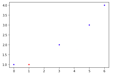
Graphical Depiction
The graph below depicts the Nearest Neighbours of the point. The the training instances are shown in blue, whereas the instance for which prediction is being made is shown in red. The x-axis shows value of input feature, whereas the y-axis shows the value of output or target value. As can be seen clearly, the value of 1 on x-axis is closest to 0, and hence the predicted value of this instance is same as that of the instance with value 0(i.e, 1).
Now, we will predict using this model for different values of input. Let’s predict the values for 2(which is closest to 3), 3.99(closest to 3), 4.01(closest to 5) and 10(closest to 6).
model.predict([[2], [3.99], [4.01], [10]])
>>>[2. 2. 3. 4.]
The output values are the target values of the instances that are closest to the new input.
Example 2
Now we will create a new model, like we did previously, but this time we will be set the value of n_neighbors to 2, so that it calculates the value of a new input by using the 2 nearest neighbours instead of just 1. The output will be computed by calculating the mean of the 2 nearest values.
model = KNeighborsRegressor(n_neighbors=2)
model.fit(X_train, y_train)
Now we will use this model to predict the value of 1.
model.predict([[1]])
Since 1 is closest to 0 and 3, the output value will be the mean of the values of 0 and 3. The output will hence be the mean of 1 and 2, which will be 1.5
>>>[1.5]
Similarly we can set the value of n_neighbors as we desire and the output will be computed as the mean of the values of n closest neighbours of the input.
Conclusion
In this blog post, we have discussed how to use the Algorithm of Nearest Neighbours in Scikit Learn. We have taken 2 examples and demonstrated how the output values differ by using different values of nearest neighbours. In this post we have taken the example of Regression for the Nearest Neighbours. In future blog posts we will talk about how the Algorithm of Nearest Neighbours in Scikit Learn can be used with Classification. We will also talk about various modifications of the standard Nearest Neighbours Algorithms in future posts.
You can find the code for this blog on Github here.