Artificial Neural Networks, or ANN, as they are sometimes called were among the very first Neural Network architectures. They are inspired by network of biological neurons in our brains. I find it very important to mention here that the Artificial Neural Networks are only inspired by the biological neurons and are not designed to model the them. Hence, an Artificial Neural Network should be considered as a Machine Learning model trying to learn a real world function instead of modelling the human brain. Artificial Neural Networks along with its variants such as CNNs and RNNs have lately been quite famous for the amazing feats they have achieved. In this blog post we will be building own own Artificial Neural Network from Scratch.
Like our last blog post, in this blog post also we will be using the Keras library which will be internally using Tensorflow as a computational engine. Following this, we will be training the Artificial Neural Network we built from scratch on the MNIST dataset after preprocessing the data. We will also compare how the this Artificial Neural Network we created from scratch fares against the Convolutional Neural Network we created from scratch in the last post. So let’s start building our own Artificial Neural Network from Scratch.
MNIST Dataset
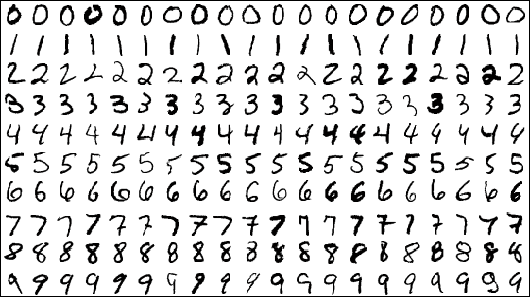
As we discussed in the last post, the MNIST dataset contains images of handwritten Hindu-Arabic numerals from 0-9. And we will be building an Artificial Neural Network from Scratch using Keras to classify these handwritten digits. The image below, Fig. 1, contains a few samples from the dataset.
Loading the Data
from tensorflow import keras
from keras.datasets import mnist
(X_train, y_train), (X_test, y_test) = mnist.load_data()
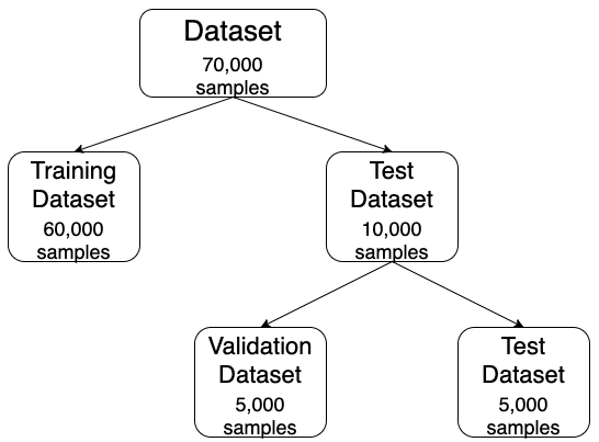
We will start by importing the Keras library and loading the data into memory. We will divide the dataset which contains 70,000 samples into the training set(X_train, y_train), which will contain 60,000 samples and the test set(X_test, y_test), which will contain 10,000 samples. Afterwards, we will divide the test set into the test set(X_test, y_test) and the validation set(X_val, y_val), which will contain 5,000 samples each. This division is also similar to the one we did in the last blog post. This is being done to ensure that we use the final test set to measure only the accuracy of the model on real world data. The diagram below, Fig. 2, shows how the data will be divided into training set, validation set, and the test set.
Creating Neural Network Model
model=keras.models.Sequential()
model.add(keras.layers.Flatten(input_shape=[28, 28]))
model.add(keras.layers.Dense(250, activation='relu'))
model.add(keras.layers.Dense(100, activation='relu'))
model.add(keras.layers.Dense(10, activation='softmax'))
We have created a model of our Artificial Neural Network(ANN). We first create a Sequential model and then we add layers to this model.
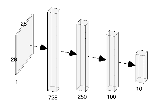
Our first layer is the Flatten layer. The flatten layer is added to the model to transform the features which are represented as a matrix(such as in an image) to a vector. The image has dimensions of 28*28, therefore the flatten layer will create a vector of length 728(28*28), one input neuron representing the value of each pixel. Next we create a Dense layer(a fully connected layer) with 250 neurons and ReLU activation function as a successor to this layer. Similarly after this we create another Dense layer with 100 neurons which also use the ReLU activation function. Lastly, we add the last layer, which is a Dense layer with 10 neurons(each one representing a separate output class- from 0 to 9). However in the last layer we use the softmax activation function instead of the ReLU. This is because we want the output to represent the probability that an input image belongs to a particular class.
A visual depiction of the model in Fig. 3.
We can get a summary for the ANN model by calling the summary method on the model.
model.summary()
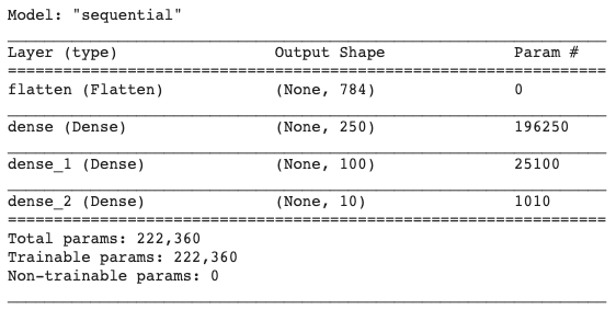
Fig 4. Summary of our ANN model
Preprocessing the Data
We will now be pre-processing the data and then feeding it to our Artificial Neural Network we just created from Scratch. This will include 3 steps which will be- normalizing the data, changing the data-type of data and lastly creating a validation set.
Normalizing the Data
As the images are grayscale, a single number between 0 and 255 can represent the value of a pixel in the image. We will be changing this scale from 0-255 to 0-1 by dividing all the values in the image by 255. This will reduce the computational load and hence will decrease the time and computational resources required for training the model.
Note– This won’t destroy any information in the image as it just changes the scale between which the numbers are present and the relative brightness will still be the same. Moreover, the original values can be recovered by changing the scale back to 0-255. This can be done by multiplying all the values by 255.
X_train=X_train/255
X_test=X_test/255
Changing the data-type of the Data
print(X_train.dtype)
>>> float64
The current data type of input samples is float64. To too will reduce to computational load and hence to decrease the time and computing resources required for training the model, we will be changing the data type for the inputs(X_train, X_test) to float32.
X_train.astype('float32')
X_test.astype('float32')
Creating Validation Set
We will create a validation set by dividing the test set into validation set and test set. We will be measuring the accuracy of the model on the validation set during training. The test set will be used only after training is completed to see how our trained model will perform in a real world scenario.
X_test, X_val=X_test[:5000], X_test[5000:]
y_test, y_val=y_test[:5000], y_test[5000:]
Compiling Model
We compile the model by calling the compile method on the model . We specify the optimizer for the model, which is the Stochastic Gradient Descent along with the loss function which is Sparse Categorical Cross-Entropy. The model is trained using this loss function and optimizer. Optionally we can also specify the metrics to be displayed during the training time, such as accuracy.
model.compile(loss='sparse_categorical_crossentropy', optimizer='sgd', metrics=['accuracy'])
Training the Model
Now, we will start the training the model. We train the model by calling fit method on the model. We provide it with the training data(the input samples X_train and output labels y_train), number of epochs(i.e, the number of times the model will iterate through the data)- which is set at 20 and the validation data(X_val and y_val). The metrics provided earlier when compiling the model, such as accuracy will be measured on this validation set after each epoch on the training set.
history=model.fit(X_train, y_train, epochs=10, validation_data=(X_val, y_val))
The fit method returns an object of the class History which we will store in the variable history. It contains important data such as the number of epochs, loss and accuracy on the training and the validation sets after each epoch. This data might be required for creating visualizations, which we will be covering in later blog posts.
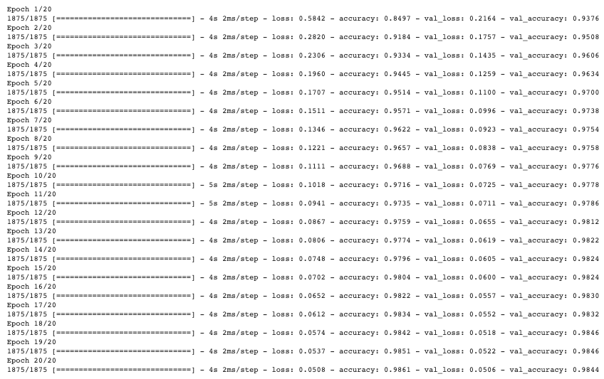
The above figure, Fig. 5. shows the value of loss and accuracy on training set and validation set at the end of each epoch.
Evaluating the Model
After 20 epochs on the training set, the accuracy on the training set is 98.61% while that on the validation set is 98.44%. But how will this model perform on real world data? To find this answer we will evaluate the accuracy of the model on test set. This should certainly give us a reasonable idea of the accuracy our model on real world data.
We evaluate the model by calling the evaluate method on the model. We provide it with the test set, i.e, X_test and y_test.
model.evaluate(X_test, y_test)
The Loss and Accuracy of the model on this test set is shown below in Fig. 6.

Conclusion
In this blog post we talked about how we can create our own Artificial Neural Network from Scratch. We created our own Artificial Neural Network from Scratch using the Keras library. We later trained this model on the MNIST dataset. Following which we evaluated our Artificial Neural Network we built from scratch on the Test Set.
The accuracy that was obtained by our Artificial Neural Network on the test set was 96.6%, which is good. But on the same dataset Convolutional Neural Networks achieved an accuracy of 98.1%. Though this may not seem like much of a difference but error rate was reduced by approximately 45% by CNNs as compared to ANNs. This is because of the fact that CNNs are better than ANNs at pattern recognition. This effect is comparatively much more visible on larger more complicated neural networks which are useful for more sophisticated tasks.
This is all that is in store for this blog post. In later blog posts we will be building many other interesting Neural Networks from scratch.
You can find the code for this blog on Github here.