Before moving further with Quantum Computing and Qiskit, it is important to learn about the differences between a Classical Computer and a Quantum Computer. In this chapter of the Qiskit Tutorial, you will learn about the differences between a Classical Computer and a Quantum Computer.
Bit vs Qubit
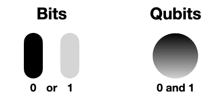
The fundamental difference between a Quantum Computer and a Classical Computer is at the most basic level of computation. In Classical Computer, the most basic level of computation is a bit. A bit can either be a 0 or a 1 at any given instance.
In Quantum Computing, we have a Qubit or a Quantum bit, the analogue of bit in Quantum Computing. Like a bit, a Qubit can either be in the state 0 or 1. However, unlike a bit, it can also be in a state of superposition, where it is simultaneously both 0 and 1. However, this state of superposition can exist only until the state of the Qubit is not measured. Once the state of the Qubit is measured, it will collapse into either 0 or 1, with different probabilities. For example, the state of a Qubit can be such that it is in superposition of states 0 and 1. However, this state of superposition will collapse into 0 or 1 upon measurement. The possibility with which a Qubit will collapse into 0 or 1 upon measurement depends on the state of the Qubit.
Classical Computer vs Quantum Computer
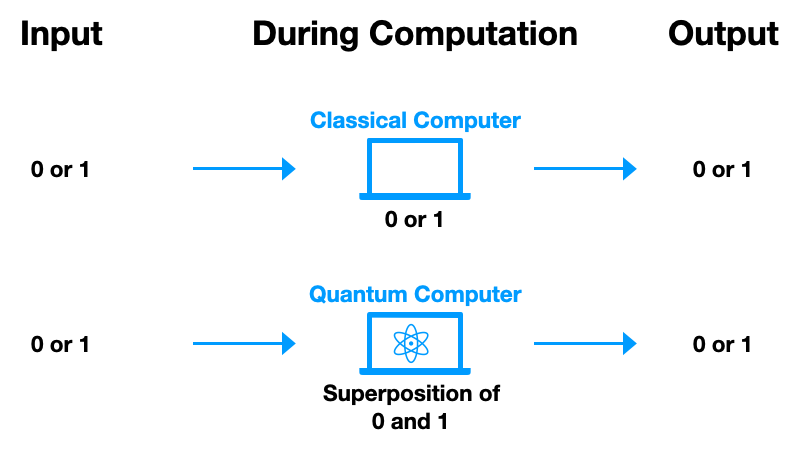
For a Classical Computer, the Input and Output, both are binary. Moreover, during computation as well, the bits are in either 0 or 1.
For a Quantum Computer, like Classical Computer, the Input and Output are both binary. But during the computation, the bits are in superposition of 0 and 1. The inputs provided to the Quantum Computer are binary. During computation, operations are applied on Qubits, like they are on bits, which can cause them to be in a state of superposition of 0 and 1. However, this state of superposition cannot be measured. Therefore, on measuring a Qubit, its state collapses into either 0 or 1. The probability with which the Qubit will collapse into 0 or 1 is dependent on the state of the Qubit when measurement is taken place, which in turn depends on the operations which were applied to the Qubit. These similarities between 0 and 1 are depicted in the figure below.
One important takeaway from the previous section is that the output of a Qubit and therefore Quantum Computer is probabilistic. But what good can probabilistic outcomes do?
Since the outcome of Qubits is probabilistic and not random, it turns out that it can have many practical applications. Running the same set of operations multiple times, you can get the Quantum Computers to solve problems that turn out to be too difficult for classical computers. These problems include problems such as factoring large numbers, which is used for Public Key Encryption and solving the Travelling Salesman Problem.
The various operations that are applied on Qubits are Quantum Gates. These Quantum Gates perform operations on the Qubits and change their state. In this tutorial, you will learn about various Quantum Gates and their effect on the Qubits. You will also learn how you can apply these Quantum Gates on your Qubits in Qiskit.
However, before moving on with Quantum Gates, it is important to learn how to represent the state of a Qubit. This is what you will be learning in the next chapter.