Convolutional Neural Networks, or CNN, as they are better known, are widely used nowadays for a variety of tasks ranging from Natural Language Processing(NLP) to Computer Vision tasks such as Image Classification and Semantic Segmentation. In this blog post, we will be building our own Convolutional Neural Network from Scratch using the Keras library. Keras is an open-source library that provides an easy to use and intuitive API. Keras can use many compute engines such as TensorFlow, Microsoft Cognitive Toolkit, Theano, or PlaidML for computation. In this particular example however, keras will internally use Tensorflow as its computational engine. Our Neural Network will be trained on MNIST Handwritten Dataset. So let’s get started with building our first Convolutional Neural Network from Scratch.
MNIST Dataset
The MNIST dataset is a very large database of handwritten Hindu-Arabic numerals(numbers from 0-9). Fig. 1. below shows a few samples of the MNIST handwritten dataset. We will be building a Convolutional Neural Network from scratch to classify which image contains which number.

Loading the Data
from tensorflow import keras
from keras.datasets import mnist
(X_train, y_train), (X_test, y_test) = mnist.load_data()
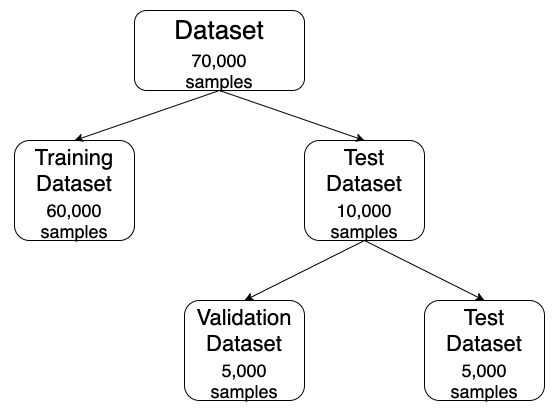
Firstly, we start by importing the Keras library and loading the dataset. For now, we have divided the dataset into 2 part, the training set (X_train, y_train) and the test set (X_test, y_test). Later, we will create 2 datasets out of the test set, namely test set (X_test, y_test) and validation set (X_val, y_val). Thus we will create 3 subsets from the original dataset(containing 70,000 samples), the training dataset(will contain 60,000 samples), the validation dataset(will contain 5,000 samples) and the test set(will contain 5,000 samples). This distribution is depicted in Fig. 2.
Creating Neural Network Model
model=keras.models.Sequential()
model.add(keras.layers.Conv2D(32, (5, 5), activation='relu', input_shape=(28, 28, 1), padding='same'))
model.add(keras.layers.MaxPool2D((2, 2)))
model.add(keras.layers.Conv2D(64, (3, 3), activation='relu'))
model.add(keras.layers.MaxPool2D((2, 2)))
model.add(keras.layers.Conv2D(128, (3, 3), activation='relu'))
model.add(keras.layers.MaxPool2D((2, 2)))
model.add(keras.layers.Flatten())
model.add(keras.layers.Dense(128, activation='relu'))
model.add(keras.layers.Dense(10, activation='softmax'))
We have created a model for our Convolutional Neural Network(CNN). We first create a Sequential Model, and later we add layers to this model.
The first layer is a convolution layer that will contain 32 filters, the value of which will be initialized randomly, and later altered according to backpropagation rule. The size of the filter is 5*5 with stride of 1*1(default size). The activation function is ReLU and the padding is same. This is followed by a a Max-Pool 2D layer with a filter size of 2*2. This again is followed by a Convolution layer and a Max-Pool 2D layer and then by another Convolution layer and a Max-Pool 2D layers of the given parameters.
This is followed by a Flatten Layer, which causes all the units in a 2D space to be represented in a 1D space as a vector. The number of units however are the same even after using the Flatten layer. This is followed by a Dense layer and finally by an output layer. The output layer uses the softmax activation function and will hence output the probabilities by default.
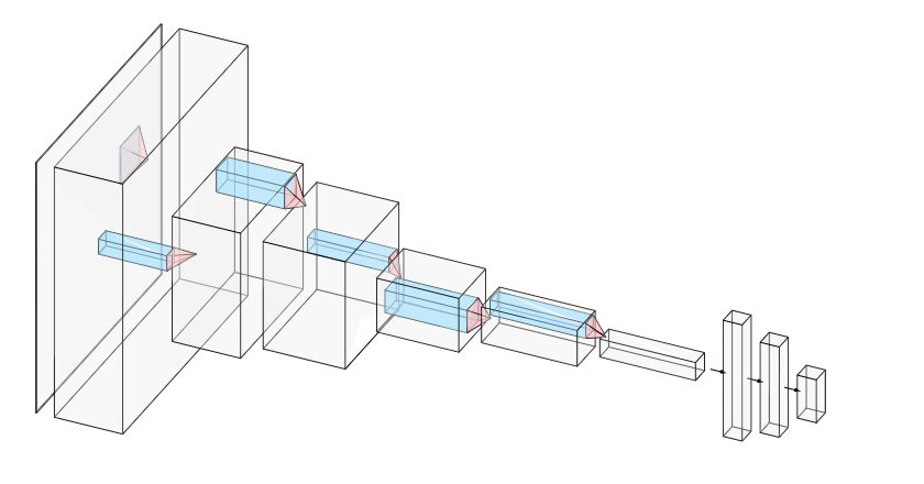
A visual depiction of the model in Fig. 3.
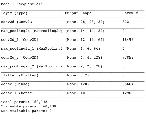
A summary for the CNN model that we produced can be obtained by calling the summary method on the model.
model.summary()
Preprocessing the Data
We will now be pre-processing the data for feeding it to our CNN. This will include 4 steps which will be reshaping the data, normalizing the data, changing the data-type of data and lastly creating a validation set.
Reshaping the Data
The current shape of the input samples is (28, 28), which specify the height and width, but not the number of channels for the image.
print(X_train.shape)
>>> (60000, 28, 28)
# Note- 60000 is the number of samples
This shape is however not suited for our CNN model. Along with height and width, we also need to have the number of channels. Since the images are grayscale images, number of channel is 1. Whereas for colour images, the number of channels is 3(one each for Red, Green and Blue). So first, we will reshape all the input samples(this includes both training set and test set) to include the number of channels too.
X_train=X_train.reshape(60000, 28, 28, 1)
X_test=X_test.reshape(10000, 28, 28, 1)
Now, the shape of the input samples is (28, 28, 1).
Normalizing the Data
The value of each pixel is represented by a number which indicates its darkness. These values range from 0 to 255. So a number 255 for a pixel will indicate that the pixel is completely black, whereas a number of 0 will indicate that the pixel is completely white. For all other numbers in between, it will indicate a shade of grey that will keep on getting darker as that number increases. We will be changing these values so that the number goes from 0 to 1 with 0 indicating complete white and 1 indicating complete black. This will not cause any problem with the image but it will make the training for the network faster. We do so by dividing the value of each pixel by 255.
X_train=X_train/255
X_test=X_test/255
Changing the data-type of the Data
The current data type of input samples is float64. This means they are stored as 64 bit float integers.
print(X_train.dtype)
>>> float64
We will be changing this to float32, i.e., 32 bit float integers. This is being done so that training is faster.
X_train.astype('float32')
X_test.astype('float32')
Creating Validation Set
We will be creating a Validation Set so that we can train our model to be optimal on the validation set and keep the test set for a just testing the real-world accuracy of the model . We will create a validation set by dividing the test set into validation set and test set.
X_test, X_val=X_test[:5000], X_test[5000:]
y_test, y_val=y_test[:5000], y_test[5000:]
Compiling Model
We compile the model by calling the compile method on the model . We also specify the optimizer for the model, the loss function to use during the training. Optionally we can also specify the metrics to be displayed during the training time, such as accuracy.
model.compile(loss='sparse_categorical_crossentropy', optimizer='sgd', metrics=['accuracy'])
Training the Model
Now, we will start the training the model. We train the model by calling fit method on the model. We provide it with the training data(the input samples X_train and output labels y_train), number of epochs(i.e, the number of times the model will iterate through the data)- which is set at 10 and the validation data(X_val and y_val). The metrics provided earlier when compiling the model, such as accuracy will be measured on this validation set after each epoch on the training set.
history=model.fit(X_train, y_train, epochs=10, validation_data=(X_val, y_val))
history will store an object of the class History, which will be returned by the fit method. It contains important parameters related to training along with other useful information related to training. But more on that in some other blog post.
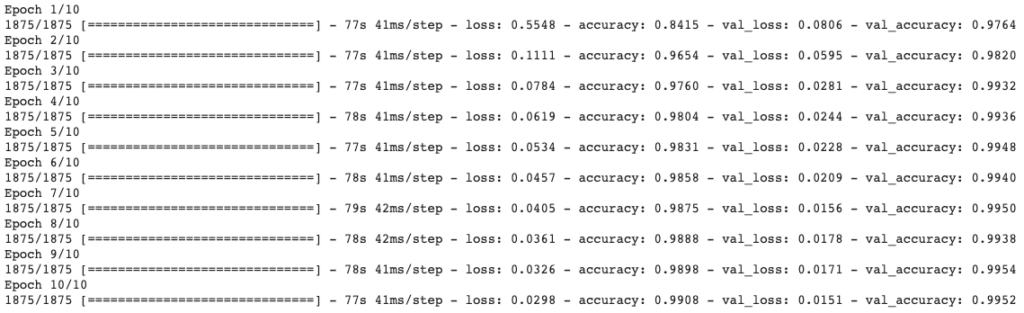
The above figure, Fig. 5. shows the value of loss and accuracy on training set and validation set at the end of each epoch.
Evaluating the Model
After 10 epochs on the training set, the accuracy on the training set is 99.08% and that on the validation set is 99.52%. But how will this model perform on real world data? To find this answer we evaluate the accuracy of the model on test set. This should give a reasonable idea of the accuracy our model on real world data.
We evaluate the model by calling the evaluate method on the model. We prove it with the test set, i.e, X_test and y_test.
model.evaluate(X_test, y_test)
The Loss and Accuracy of the model on this test set is shown below in Fig. 6.

Conclusion
In this blog post we talked about how we can create our own Convolutional Neural Network from Scratch. We created our own Convolutional Neural Network from Scratch using the Keras library. We later trained this model on the MNIST dataset. This was followed by an evaluation of our Convolutional Neural Network built from scratch using the Test Set.
This is all that is in store for this blog post. In later blog posts we will be building many other interesting Neural Networks from scratch.
You can find the code for this blog on Github here.