Self Supervised Learning, or SSL is a really hot topic in the field of Machine Learning and Deep Learning at the moment. You would have definitely come across the term in conferences, blogs, or in various other discussion groups or somewhere else by now. Self Supervised Learning is a very promising approach to training Neural Networks with limited labeled datasets. Limited quantity of labeled data has been the roadblock for training Neural Networks for a really long time. This explains why everyone wants to get in on the action. In this blog post, I will talk about implementing an approach to Self Supervised Learning, known as Pretext Training using Keras.
If you do not know what Self Supervised Learning is, I have written a blog post explaining briefly about Self Supervised Learning. You can check out the blog post here. I recommend that you go through the blog post if you have absolutely no idea about Self Supervised Learning because a basic understanding of the same would be required for going through this blog post. If you do not know about Pretext training, you can check out my blog on Pretext Training here. The task that will be used for Pretext Training will be performing the amount of rotation for images. There are various pretext tasks that you can perform, I have written a blog about Pretext Training tasks, including Image Rotation Pretext Training task about which you can read here.
If you have an idea of Self Supervised Learning, Pretext Training, and Keras then you should not have any difficulty with following along this blog. You can check out to blog on how to build and train a Convolutional Neural Network to classify images of handwritten numbers(MNIST) here. This example should be sufficient for you to get the basics right and follow along with this blog post. This blog will mostly be about the code and its explanation. Don’t bother about copying the code, you will find the link to the Github notebook for this code at the end of this blog.
Importing Libraries
What’s the first thing we do before we begin to code? That’s right! Import all the necessary libraries. So let’s do that first.
# Importing Libraries

import numpy as np
import pandas as pd
import matplotlib
import matplotlib.pyplot as plt
import tensorflow as tf
from tensorflow import keras
The Dataset
For this example, we will be using the Fashion MNIST Dataset. The dataset contains 28 * 28 pixels images of various types of fashion items including tops, bottoms, boots, etc. The dataset consists of a total of 70,000 images. Out of these 70,000 images, a total of 50,000 will be used for pretext training out of which 40,000 will be used for training and 10,000 as validation dataset. Another 10,000 will be used for training the model on the final downstream task, and 10,000 images each will be used as validation and test datasets for the downstream task.
Loading Data
The most import thing to perform Machine Learning is to have data. For this example we will be making use of the Fashion MNIST dataset that we will load by using the API provided by Keras.
data=keras.datasets.fashion_mnist

# Getting the data
(X_train, y_train), (X_test, y_test) = data.load_data()
Data Preprocessing and Splitting
It is important to preprocess the dataset and split it into Training(X_train, y_train), Validation(X_val, y_val) and Testing Dataset(X_test, y_test).
# Normalizing the dataset

X_train = X_train/255
X_test = X_test/255


# Splitting the test dataset into validation and test dataset
X_val = X_test[:5000]
y_val = y_test[:5000]

X_test = X_test[5000:]
y_test = y_test[5000:]
Since we will be using a pretext task, we will create an un-labeled dataset for the pretext task from the training dataset. This un-labeled dataset will not be used for training the model on a downstream task.
The entire training dataset contains 60,000 images. In this example, we will be creating an un-labeled dataset of 50,000 images which will be used for pretext training(X_unlabeled). We will be separating the other 10,000 images to train out Neural Network on the Downstream task(X_labeled, y_labeled).
# Creating a un-labeled dataset from training dataset
X_unlabeled = X_train[10000:]

# Creating a labeled dataset from training dataset
X_labeled = X_train[:10000]
y_labeled = y_train[:10000]Note– Notice that labels for the un-labeled data will not be used and hence are not being stored.
Creating Pseudo Target Features for Pretext Training Dataset
Now that we have created an un-labeled dataset, the next step is to create Pseudo-targets or pseudo-labels for this un-labeled dataset. These pseudo targets depends on the pretext task you are performing. Since we are predicting the rotation of images, we will rotate the dataset by 0, 90, 180, or 270 degrees and assign corresponding pseudo-labels to them.
# X_train_0 dataset will contain images rotated by 0 degrees(No rotation)
X_train_0=X_unlabeled.copy()

# X_train_90 dataset will contain images rotated by 90 degrees
X_train_90=np.rot90(X_unlabeled, axes=(1,2))

# X_train_180 dataset will contain images rotated by 180 degrees
X_train_180=np.rot90(X_unlabeled, 2, axes=(1,2))

# X_train_270 dataset will contain images rotated by 270 degrees
X_train_270=np.rot90(X_unlabeled, 3, axes=(1,2))

# Assigning pseudo-labels to rotated image datasets
y_train_0=np.full((50000), 0)
y_train_90=np.full((50000), 1)
y_train_180=np.full((50000), 2)
y_train_270=np.full((50000), 3)
Next, we concatenate the various datasets that contains different amount of rotations together and perform the same for their pseudo-labels. This creates a concatenated dataset for all the data with different rotations(X_train_unlabeled_full, y_train_unlabeled_full).
# Concatenating Datasets
X_train_unlabeled_full=np.concatenate((X_train_0, X_train_90, X_train_180, X_train_270), axis=0)
y_train_unlabeled_full=np.concatenate((y_train_0, y_train_90, y_train_180, y_train_270), axis=0)
Next, we have to shuffle the concatenated dataset so that the samples of various rotations are uniformly distributed over the entire dataset. But the order of shuffling needs to be the same for both, the input features(X_train_unlabeled_full) and the pseudo target features(y_train_unlabeled_full). We create a function unison_shuffled_copies which will do this task.
# The function will distribute the samples uniformly over dataset
def unison_shuffled_copies(a, b):
    assert len(a) == len(b)
    p = np.random.permutation(len(a))
    return a[p], b[p]
We pass the concatenated input features and pseudo-labels to the unison_shuffled_copies() function to get a shuffled version of the dataset(X_train_unlabeled_full_shuffled, y_train_unlabeled_full_shuffled).
# Randomly shuffling the concatenated dataset
X_train_unlabeled_full_shuffled, y_train_unlabeled_full_shuffled = unison_shuffled_copies(X_train_unlabeled_full, y_train_unlabeled_full)
Training a Convolutional Neural Network on Pretext Task
Now that we have the un-labeled dataset ready along with pseudo-labels, we can create a Convolutional Neural Network and train the model on the pretext task of predicting the rotation of the images.
We start by creating a convolutional Neural Network.
# Creating a Convolutional Neural Network
model = keras.models.Sequential([
        keras.layers.Conv2D(64, 7, activation="relu", padding="same",
                            input_shape=[28, 28, 1]),
        keras.layers.MaxPooling2D(2),
        keras.layers.Conv2D(128, 3, activation="relu", padding="same"),
        keras.layers.Conv2D(128, 3, activation="relu", padding="same"),
        keras.layers.MaxPooling2D(2),
        keras.layers.Conv2D(256, 3, activation="relu", padding="same"),
        keras.layers.Conv2D(256, 3, activation="relu", padding="same"),
        keras.layers.MaxPooling2D(2),
        keras.layers.Flatten(),
        keras.layers.Dense(128, activation="relu"),
        keras.layers.Dropout(0.5),
        keras.layers.Dense(64, activation="relu"),
        keras.layers.Dropout(0.5),
        keras.layers.Dense(4, activation="softmax")
])
Next, we compile the model. While compiling, we set the loss function to Sparse Categorical Cross-Entropy and the Optimizer to Stochastic Gradient Descent.
# Compiling the model
model.compile(loss="sparse_categorical_crossentropy", optimizer="sgd", metrics=["accuracy"])
We split the Training dataset into Validation Set(X_rot_val, y_rot_val) and Training Set(X_rot_train, y_rot_train) for the pretext task. Since we are training the model on pretext task on which the model will not be evaluated, we are not taking a test dataset. This should not lead to any issues until and unless there is serious over-fitting. However, it might be a good practice to take out a testing dataset and evaluate the model on it.
# Creating Validation and Test Dataset for Pretext Task
X_rot_val, X_rot_train = X_train_unlabeled_full_shuffled[:10000], X_train_unlabeled_full_shuffled[10000:]
y_rot_val, y_rot_train = y_train_unlabeled_full_shuffled[:10000], y_train_unlabeled_full_shuffled[10000:]
The inputs need to be reshaped so that their shape is the same as expected by the Neural Network.
# Reshaping the Inputs
X_rot_val=X_rot_val.reshape(-1, 28, 28, 1)
X_rot_train=X_rot_train.reshape(-1, 28, 28, 1)
Finally, the time to train our model has come. We call the fit() method and pass it the training and validation datasets and let it run for 5 epochs.
# Training the model on Pretext Task
history = model.fit(X_rot_train, y_rot_train, epochs=5, validation_data=(X_rot_val, y_rot_val))
Training Model on Downstream Task
Now that we have out model trained on the Pretext Task, it’s time to train it on the downstream task on which it will be actually evaluated.
We remove the final layer and append a new final layer, a one that has labels corresponding to the downstream task.
# Removing the top layer and addding a new top layer
model.pop()
model.add(keras.layers.Dense(10, name='dense_3', activation='softmax'))
Convolutional Layers are really good at capturing patters and applying it to other tasks. It is for this reason that Convolutional Neural Networks perform very well when using Transfer Learning. However, Dense Layers fail to apply their learned patterns to other tasks. It is for this reason, that it becomes important to retrain the Dense Layers while the Convolutional Layers are freezed.
# Freezing the Convolutional Layers while keeping Dense layers as Trainable
for layer in model.layers:
    if layer.name in ['dense_3', 'dense_1', 'dense', 'dropout', 'dropout_1']:
      layer.trainable=True
    else:
      layer.trainable=False
Again, we need to reshape the inputs to the Neural Network to a shape that is expected by our Neural Network.
# Reshaping the Inputs
X_labeled=X_labeled.reshape(-1, 28, 28, 1)
X_val=X_val.reshape(-1, 28, 28, 1)
X_test=X_test.reshape(-1, 28, 28, 1)
We compile the model and set the loss to Sparse Categorical Cross-Entropy and Optimizer to Stochastic Gradient Descent, but this time for the final downstream task.
# Compiling the model
model.compile(loss="sparse_categorical_crossentropy", optimizer="sgd", metrics=["accuracy"])
Now we train the model on the final downstream task by using a small labeled dataset(X_labeled, y_labeled) for a total of 10 epochs. In each epoch, we check the accuracy of the model on the validation dataset(X_val, y_val).
# Training the model on Downstream Task
history = model.fit(X_labeled, y_labeled, validation_data=(X_val, y_val), epochs=10)
The image below shows how the training and validation losses and accuracy fare over various epochs.
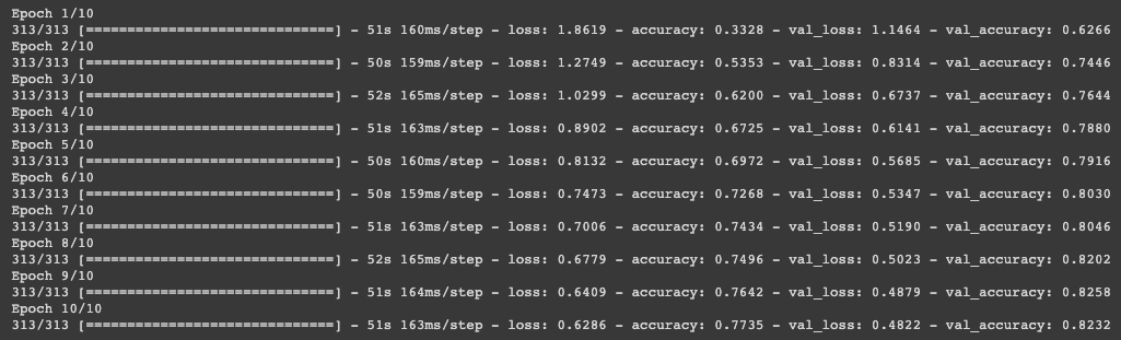
Finally, we evaluate the accuracy of the model on test dataset.
# Evaluating the model on the Test set
model.evaluate(X_test, y_test)
The accuracy of the model on test dataset for this particular example at the time of doing it was found to be 84.32%

In this blog post, we learned how to perform a pretext task of predicting the rotation of images by using a un-labeled data followed by training the model on a downstream task using Keras. In my next blog post I will talk about how this model trained by using a pretext task before the final downstream task compares to a similar model that is trained only on the labeled data of the same size. You can check out the next blog post on comparing the models trained with Pretext Learning and Supervised Learning over here.
You can find the Jupyter notebook for this example on Github over here.